Molecular Dynamics Simulations of Hysteresis Loops for BaTiO3 Ferroelectric Thin-Film Capacitors Using the feram Code

How to use Slidy

This presentation is written with Slidy http://www.w3.org/Talks/Tools/Slidy/ . Use Firefox web browser.

• Advance to next slide with mouse click or [Space]
• Move forward/backward between slides with [Left], [Right], [Pg Up] and [Pg Dn] keys
• [Home] key for first slide, [End] key for last slide
• The [C] key for an automatically generated table of contents (or click on "contents" on the toolbar)
• Function [F11] toggles between the full screen mode and the normal mode
• [F] key toggles the display of the tool bar below.
• [A] key toggles the presentation mode and the printing mode
• [S] and [B] keys can control the size of fonts

What is ferroelectric?

Properties of ferroelectrics, such as BaTiO${}_3$, PbTiO${}_3$, KNbO${}_3$, LiNbO${}_3$, LiTaO${}_3$, SrTiO${}_3$, Pb(Zr${}_{(1-x)}$Ti${}_x$)O${}_3$ (PZT), etc..

Non-volatile ferroelectric memory (FeRAM)

Schematic device configurations of two types of FeRAM (a) 1-transistor and 1-capacitor (1T1C) type and (b) 1-transistor (1T) type. (c) and (d) are their circuit diagrams, respectively.

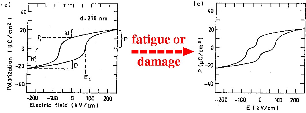
Ferroelectric thin-film capacitors (background of this study)

• Various applications of ferroelectric thin-films:
  • multilayer capacitors
  • nonvolatile FeRAMs
  • nanoactuators
• Down-sizing of FeRAMs (nano-capacitors of ferroelectric thin films) is highly demanded.
• Epitaxially constraint ferroelectric films made by PLD.
• Effect of imperfect screening of electrodes is NOT well understood.
  • [M. Dawber et al.: J. Phys. Condes. Matter 15, L393 (2003)]
• Fatigue causes damages in polarization behaviors of ferroelectric capacitors.

After [J. F. Scott: Ferroelectric Memories (Springer, 2000)].

Dynamics, nanosize effects and temperature dependences

• Dynamics of ferroelectric thin-film capacitors:
  • Hysteresis loop
  • Polarization switching
  • Dynamics of domain wall
• Their nanosize effects and temperature dependences remain poorly known.
  • Experimentally, in situ observations are difficult.
  • Theoretically,
    • The long-range Coulomb interaction limits the size and time of molecular-dynamics (MD) simulations.
    • How to include depolarization fields caused by imperfect electrodes was unclear.

After [Fong et al.: Science 304, 1650 (2004)]. Ultra thin films ($<4$ layers) may not have spontaneous polarization.

Purpose of this study

• Development of fast molecular dynamics (MD) code which can simulate ferroelectric thin-film capacitors for a realistic system size (up to 100 nm) and a realistic time span ($>$ 1 ns).
• Clarify the effect of dead layers between ferroelectrics and electrodes.
• Predict the effect of the compressive strain arising from epitaxial constraints.

$\to$ We develop "feram" code.

Features of feram program

• Scientific features
  • Molecular dynamics (MD) simulation with first-principles-based effective Hamiltonian
  • $AB$O₃-type perovskite ferroelectrics and relaxors
  • Uses supercell; ($AB$O₃)${}_N$, $N=32\times 32\times 512$ $\Rightarrow$ 2,621,440 atoms
  • Coarse-graining; reduction of the number of degree of freedom
  • Long-range dipole-dipole interaction is treated in reciprocal-space; k-locality of the force matrix
  • Applications:
    • Phase transition of bulk ferroelectrics
    • Capacitor, ferroelectric thin film is sandwiched between short-circuited electrodes

• Technical features
  • Fast
    • FFTW library version 3 http://www.FFTW.org/
    • Parallelized with OpenMP http://www.OpenMP.org/
  • Multi-platform
    • Linux PC
    • HITACHI SR11000 Super Technical Server
    • SONY PLAYSTATION3 (ongoing)
  • Object oriented programming (OOP) in Fortran 2003
  • GNU autotools http://www.gnu.org/software/autoconf/
  • Free software (GPLv3) http://loto.sf.net/feram/

Soft-mode displacements of perovskite type ferroelectrics ABO₃

Coupling between atomic displacements and strains. After [T. Hashimoto, T. Nishimatsu et al.: Jpn. J. Appl. Phys. 43, 6785 (2004)].

$$u_{\alpha }^2=\{v_{\alpha }^A{\}}^2+\{v_{\alpha }^B{\}}^2+\{v_{\alpha }^{{\mathrm{O}}_{\mathrm{I}}}{\}}^2+\{v_{\alpha }^{{\mathrm{O}}_{\mathrm{I}\mathrm{I}}}{\}}^2+\{v_{\alpha }^{{\mathrm{O}}_{\mathrm{I}\mathrm{I}\mathrm{I}}}{\}}^2$$

Potential surface of the zone-center distortion for BaTiO₃

Calculated potential surfaces of the zone-center distortion for BaTiO₃ with various $E_{\mathrm{x}\mathrm{c}}$.

Coarse-graining

• Real perovskite-like system has $15N+6$ degree of freedom
  • $N$ unit cells in a supercell
  • 5 atoms per unit cell
  • Each atom can move along 3 directions
  • 6 components of strain

• Simplified model has $6N+6$ degree of freedom
  • Define 1 dipole $Z^{*}\mathit{u}\left(\mathit{R}\right)$ per unit cell
  • 1 acoustic displacement (Inhomogeneous strain) $\mathit{w}\left(\mathit{R}\right)$ per unit cell

First-principles effective Hamiltonian for a supercell

Supercell of ($AB$O₃)${}_N$ with $\left\{\mathit{u}\right(\mathit{R}\left)\right\}$ and $\left\{\mathit{w}\right(\mathit{R}\left)\right\}$: $$H^{\mathrm{e}\mathrm{f}\mathrm{f}}=\frac{M_{\mathrm{d}\mathrm{i}\mathrm{p}\mathrm{o}\mathrm{l}\mathrm{e}}^{*}}{2}\sum _{\mathit{R},\alpha }{\stackrel{\cdot }{u}}_{\alpha }^2\left(\mathit{R}\right)+\frac{M_{\mathrm{a}\mathrm{c}\mathrm{o}\mathrm{u}\mathrm{s}\mathrm{t}\mathrm{i}\mathrm{c}}^{*}}{2}\sum _{\mathit{R},\alpha }{\stackrel{\cdot }{w}}_{\alpha }^2\left(\mathit{R}\right)+V^{\mathrm{s}\mathrm{e}\mathrm{l}\mathrm{f}}\left(\right\{\mathit{u}\left\}\right)+V^{\mathrm{d}\mathrm{p}\mathrm{l}}\left(\right\{\mathit{u}\left\}\right)+V^{\mathrm{s}\mathrm{h}\mathrm{o}\mathrm{r}\mathrm{t}}\left(\right\{\mathit{u}\left\}\right)+V^{\mathrm{e}\mathrm{l}\mathrm{a}\mathrm{s},\mathrm{h}\mathrm{o}\mathrm{m}\mathrm{o}}({\eta }_1,...,{\eta }_6)+V^{\mathrm{e}\mathrm{l}\mathrm{a}\mathrm{s},\mathrm{i}\mathrm{n}\mathrm{h}\mathrm{o}}\left(\right\{\mathit{w}\left\}\right)+V^{\mathrm{c}\mathrm{o}\mathrm{u}\mathrm{p},\mathrm{h}\mathrm{o}\mathrm{m}\mathrm{o}}\left(\right\{\mathit{u}\},{\eta }_1,...,{\eta }_6)+V^{\mathrm{c}\mathrm{o}\mathrm{u}\mathrm{p},\mathrm{i}\mathrm{n}\mathrm{h}\mathrm{o}}\left(\right\{\mathit{u}\},\{\mathit{w}\left\}\right)-Z^{*}\sum _{\mathit{R}}ℰ\cdot \mathit{u}\left(\mathit{R}\right)$$

Snapshot of the supercell. Strengths and directions of $\left\{\mathit{u}\right(\mathit{R}\left)\right\}$ are indicated with arrows. red and blue colors represent $+z$-polarized and $-z$-polarized sites.

Self potential of a local dipole

$$V^{\mathrm{s}\mathrm{e}\mathrm{l}\mathrm{f}}\left(\mathit{u}\right)={\kappa }_2{u}^2+\alpha u^4+\gamma (u_y^2{u}_z^2+u_z^2{u}_x^2+u_x^2{u}_y^2)$$

where

$$u^2=u_x^2+u_y^2+u_z^2.$$

Schematic illustration of self potential of a local dipole. Double well is made by the fourth order terms of u.

Dipole-dipole interaction

In the effective Hamiltonian, dipole-dipole interactions are separated into the long-rage term and the short-range term.

Long-range: $$V^{\mathrm{d}\mathrm{p}\mathrm{l}}\left(\right\{\mathit{u}\left\}\right)=\frac{1}{2}\sum _{i=1}^N\sum _{\alpha }\sum _{j=1}^N\sum _{\beta }{u}_{\alpha }\left({\mathit{R}}_i\right){\mathrm{\Phi }}_{\alpha \beta }\left({\mathit{R}}_{ij}\right)u_{\beta }\left({\mathit{R}}_j\right),$$

$${\mathrm{\Phi }}_{\alpha \beta }\left({\mathit{R}}_{ij}\right)=\frac{Z^{*2}}{{\epsilon }_{\mathrm{\infty }}}\sum _{\mathit{n}}{}^{\prime }\frac{{\delta }_{\alpha \beta }-3\left(\widehat{{\mathit{R}}_{ij}+\mathit{n}}{)}_{\alpha }\right(\widehat{{\mathit{R}}_{ij}+\mathit{n}}{)}_{\beta }}{|{\mathit{R}}_{ij}+\mathit{n}{|}^3},$$

$\mathit{n}$ is the supercell lattice vector: $$n_{\alpha }=\cdots ,-2L_{\alpha }{a}_0,-L_{\alpha }{a}_0,0,L_{\alpha }{a}_0,2L_{\alpha }{a}_0,\cdots$$

Short-range: $$V^{\mathrm{s}\mathrm{h}\mathrm{r}\mathrm{t}}\left(\right\{\mathit{u}\left\}\right)=\frac{1}{2}\sum _{i=1}^N\sum _{\alpha }\sum _j^{3\mathrm{n}\mathrm{n}}\sum _{\beta }{u}_{\alpha }\left({\mathit{R}}_i\right)J_{ij,\alpha \beta }{u}_{\beta }\left({\mathit{R}}_j\right)$$ $J_{ij,\alpha \beta }=J_k$: Short-range interaction matrix ($k=1,\cdots ,7$)

Forces on dipoles are calculated in the reciprocal space

Simplified flow chart for calculating forces on dipoles. Fast Fourier transformation (FFT) and inverse FFT (IFFT) enable the rapid calculation of long-range dipole-dipole interactions. You can reduce computational time from $O\left(N^2\right)$ to $O\left(N\log N\right)$.

Long-range dipole-dipole interaction

Long-range interaction energy per unit cell is plotted in the first Brillouin zone for the simple cubic crystal. Only with dipole-dipole interaction, the minimum is at the M point, i.e., the checker-board-type antiferroelectric order is most stable.

Long-range + short-range interaction

By introducing short-range interaction, the minimum come to the $\mathrm{\Gamma }$ point, i.e., the ferroelectric order is most stable.

First Brillouin zone for simple cubic crystals

First Brillouin zone for simple cubic crystals.

LO-TO splitting

LO-TO splitting is the ion version of the plasma frequency.

Schematic illustration of longitudinal oscillation of a dielectric thin film. Polarization $P_z=Z^{*}{u}_z/\mathrm{\Omega }$ perpendicular to the film causes surface charges $\pm P_z$. The surface charges result in depolarization field $E_{\mathrm{d}}=-4\pi P_z$ in the film. This depolarization field causes restoring force $F=-4\pi Pz{Z}^{*}{u}_z=-4\pi Z^{*2}{u}_z^2/\mathrm{\Omega }$ on $u_z$.

Boundary condition for capacitors

Ferroelectrics are sandwiched between short-circuited perfect electrodes (a) and imperfect electrodes (b). In (a) depolarization field $E_{\mathrm{d}}=0$, but in (b) $E_{\mathrm{d}}=-4\pi P_z\frac{d}{l+d}$.

Parameters for BaTiO₃ Hamiltonian (input file)

• [King-Smith and Vanderbilt: Phys. Rev. B 49, 5828 (1994)]
• [Zhong, Vanderbilt, and Rabe: Phys. Rev. B 52, 6301 (1995)]

#--- Method, Temperature, and mass ---------------
method = 'md'
   # 'md' - Molecular Dynamics with Nose-Poincare thermostat (Canonical ensemble)
   # 'lf' - Leap Frog (Microcanonical ensemble)
   # 'hl' - Hysteresis Loop
   # 'mc' - Monte Carlo (not implemented yet)
GPa = -5.0
kelvin = 300
mass_amu = 39.0       # Required for MD
Q_Nose = 1.0

#--- System geometry -----------------------------
bulk_or_film = 'bulk'
L = 32 32 32
a0 =  3.94         lattice constant a0 [Angstrom]

#--- Time step -----------------------------------
dt = 0.002 [ps]
n_thermalize =  40000
n_average    =  10000
n_coord_freq =   5000     Write a snapshot to the disk every 5000 steps

#--- On-site (Polynomial of order 4) -------------
P_kappa2 =    5.502  [eV/Angstrom^2] # P_4(u) = kappa2*u^2 + alpha*u^4
P_alpha  =  110.4    [eV/Angstrom^4] #  + gamma*(u_y*u_z+u_z*u_x+u_x*u_y),
P_gamma  = -163.1    [eV/Angstrom^4] # where u^2 = u_x^2 + u_y^2 + u_z^2

#--- Inter-site ----------------------------------
j = -2.648 3.894 0.898 -0.789 0.562 0.358 0.179    j(i) [eV/Angstrom^2]

#--- Elastic Constants ---------------------------
B11 = 126.
B12 =  44.9
B44 =  50.3  [eV]

#--- Elastic Coupling ----------------------------
B1xx = -211.   [eV/Angstrom^2]
B1yy =  -19.3  [eV/Angstrom^2]
B4yz =   -7.75 [eV/Angstrom^2]

#--- Dipole --------------------------------------
init_dipo_avg = 0.00 0.00 0.00   [Angstrom]  # Average   of initial dipole displacements
init_dipo_dev = 0.02 0.02 0.02   [Angstrom]  # Deviation of initial dipole displacements
Z_star       = 9.956
epsilon_inf   = 5.24

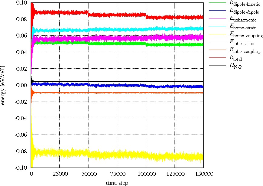
Time evolution and fluctuation

Energy versus time-step plot of a cooling simulation. You can see Nose-Poincare Hamiltonian remains zero.

Results: Monte Carlo (MC) vs. Molecular Dynamics (MD)

feram is a molecular dynamics (MD) program for bulk and thin-film ferroelectrics.

Simulations of bulk BaTiO₃ with MC and MD. Horizontal axis is temperature. Vertical axis is strain. While Monte Carlo steps do NOT have physical meaning, MD simulation steps have a physical meaning of the time evolution. Cooling and heating MD simulation can show hysteresis in temperature clearly.

Experimentally observed one after [H. E. Kay and P. Vousden: Philos. Mag. 40, 1019 (1949)]. The relatively weak first-order nature of the cubic-to-tetragonal phase transition can be compared with the first-order tetragonal-to-orthorhombic and orthorhombic-to-rhombohedral phase transitions.

Dielectric constants can be calculated from fluctuations

Temperature dependence of three components of strain and relative dielectric constant of bulk BaTiO₃. Three phase transitions are clearly seen. Dielectric constants can be calculated from fluctuations of dipoles.

Heating-up and cooling-down simulations of ferroelectric capacitors

Animations of horizontal slices of heating-up and cooling-down simulations for BaTiO₃ thin-film capacitors with short-circuited electrodes under 1% in-plane biaxial compressive strain. The +z-polarized and −z-polarized sites are denoted by red open squares and blue filled squares, respectively. Used supercell sizes are Lx×Ly×Lz = 40×40×2(l+d) .

• (a) l=15, d=1
  • heating-up
  • cooling-down
• (b) l=31, d=1
  • heating-up
  • cooling-down
• (c) l=127, d=1
  • heating-up
  • cooling-down
• (d) l=255, d=1
  • heating-up (coming soon)
  • cooling-down
• (e) l=32, d=0
  • heating-up
  • cooling-down

Single domain structures and striped domain structures

Snapshots at $T=100$ K in heating-up ((a)) and cooling-down ((b) and (c)) simulations of ferroelectric thin-film capacitors of $l=15$ with $d=1$. (a) and (b) are horizontal slices. (c) is a vertical cross section.

Thinner film has finer domain structure to avoid stronger depolarization field

Horizontal slices of domain structures in capacitors of epitaxial BaTiO₃ thin-film with imperfect electrodes $32\times 32\times (l=7,15,31,63,127and255,d=1$). Thinner film has finer domain structure to avoid stronger depolarization field $E_{\mathrm{d}}=-4\pi P_z\frac{d}{l+d}$.

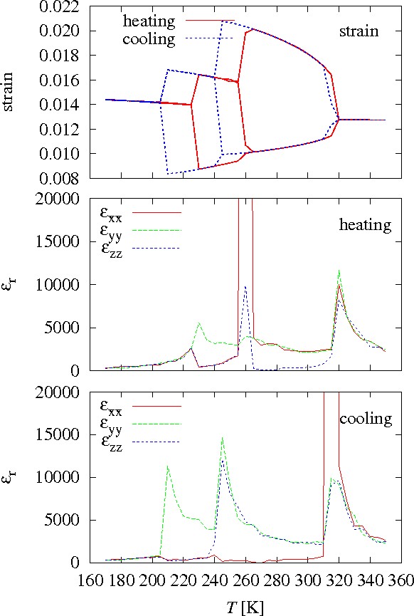
Temperature dependence of polarizations of thin-film capacitors

Uniformly polarized structure and striped domain structure

Almost uniformly polarized structure ((a) and (b)) and striped domain structure ((c) and (d)) of thin-film BaTiO₃ capacitors of $32\times 32\times (l=15,d=1)$. There is thermally unhoppable bistability between these two structure.

(1) On SrRuO₃ or Pt metallic substrate, (2) grow BaTiO₃ thin and thick thin films, (3) cover them with the metal, (4) if you use x-ray or whatever, (5) you may observe deference of fineness in their domain structures.

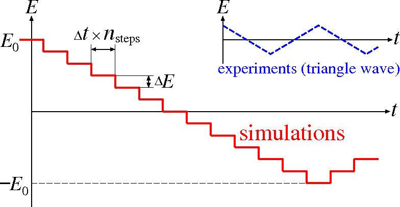
Applied external electric field

Schematic illustrations of triangle-wave electric field used to measure ferroelectric hysteresis loops experimentally (inset) and in the present simulations.

Latest version of feram can apply smooth triangle-wave electric field.

Temperature dependence of hysteresis loops for bulk BaTiO₃

Temperature dependence of hysteresis loops for bulk BaTiO₃. The phase transition from paraelectric phase to ferroelectric phase is clearly seen.

Hysteresis loops for epitaxially constrained and "free" BaTiO₃ film capacitors

Calculated hysteresis loops for capacitors with (a) epitaxially constrained films, and (b) ``free'' films of various thickness $l$ and with dead layer $d$ at 100 K.

Out-of-plane polarization is no longer the ground state

Vertical cross section of a simulated ferroelectric "free" film capacitor with a single dead layer; 16 x 16 x (l=63, d=1). The snapshot was taken at the point marked "x". The projection of the dipole moments onto the xz-plane are indicated with arrows.

Epitaxially constrained film vs. "free" film (again)

Schematic comparison between the epitaxially constrained film and the ``free'' film. In the epitaxially constrained film, switching may have to climb over a potential barrier, but, in the ``free'' film, dipoles can be easily rotated and switching can go around a valley of the potential.

Future plan with the feram code: Molecular dynamics simulations of relaxors

Relaxors Pb$B_x^{\prime }$$B_{1-x}^{\prime \prime }$O${}_3$: Pb${}^{2+}$

• Pb(Sc${}_{1/2}$Nb${}_{1/2}$)O${}_3$ (PSN): Sc${}^{3+}$, Nb${}^{5+}$
• Pb(Sc${}_{1/2}$Ta${}_{1/2}$)O${}_3$ (PST): Sc${}^{3+}$, Ta${}^{5+}$
• Pb(Mg${}_{1/3}$Nb${}_{2/3}$)O${}_3$ (PMN:) Mg${}^{2+}$, Nb${}^{5+}$
• $(1-x)$Pb(Mg${}_{1/3}$Nb${}_{2/3}$)O${}_3$-xPbTiO${}_3$ (PMN-$x$PT): Mg${}^{2+}$, Nb${}^{5+}$, Ti${}^{4+}$
• Pb(Mg${}_{1/3}$Ta${}_{2/3}$)O${}_3$ (PMT): Mg${}^{2+}$, Ta${}^{5+}$
• Pb(Zn${}_{1/3}$Nb${}_{2/3}$)O${}_3$ (PZN): Zn${}^{2+}$, Nb${}^{5+}$

The averaged valence number of B-site ions $B_x^{\prime }$ and $B_{1-x}^{\prime \prime }$ is $4+$.

Frequency dependence of dielectric constant of relaxors

After [Takaaki Tsurumi, Kouji Soejima, Toshio Kamiya and Masaki Daimon: Jpn. J. Appl. Phys. 33, 1959-1964 (1994)]

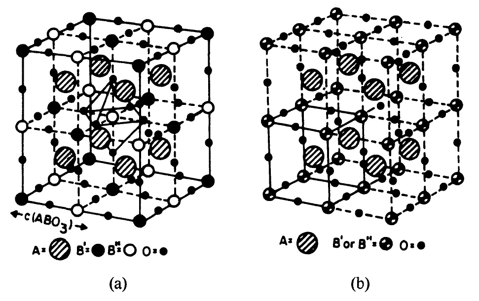
Crystal structures of relaxors

(a) Ordered B-site structure of $A{B}_x^{\prime }{B}_{(1-x)}^{\prime \prime }$O${}_3$. In the case of Pb(Sc${}_{1/2}$Nb${}_{1/2}$)O${}_3$, Sc and Nb has the NaCl structure. In the case of Pb(Mg${}_{1/3}$Nb${}_{2/3}$)O${}_3$, the Na-site is randomly occupied by Mg${}_{1/3}$Nb${}_{1/6}$ and the Cl-site is occupied by Nb${}_{1/2}$. (b) Disordered structure. B-sites is occupied by $B^{\prime }$ and $B_{(1-x)}^{\prime \prime }$ randomly. After [C. A. Randall and A. S. Bhalla: Jpn. J. Appl. Phys. 29, 327-333 (1990)].

Local field on Pb-site

Displacement of Pb is the main source of dipole moment.

Symmetric potential around Pb at the chemically ordered region (COR). Asymmetric one at the chemically disordered region (CDR).

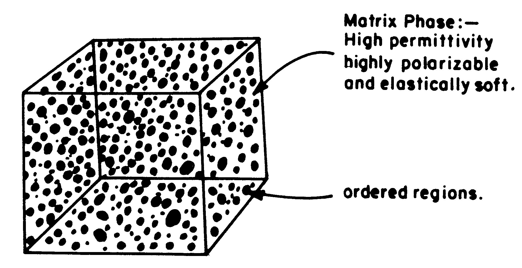
Chemically ordered and disordered regions of relaxors

The quenched sample has chemically ordered regions (∼100Å) in a chemically disordered matrix. After [C. A. Randall and A. S. Bhalla: Jpn. J. Appl. Phys. 29, 327-333 (1990)].

Modeling of relaxors

Schematic illustration of modeling of relaxor. Bubble-like Chemically ordered regions (COR, red symmetric double wells) is created in a chemically disordered matrix (blue asymmetric double wells)

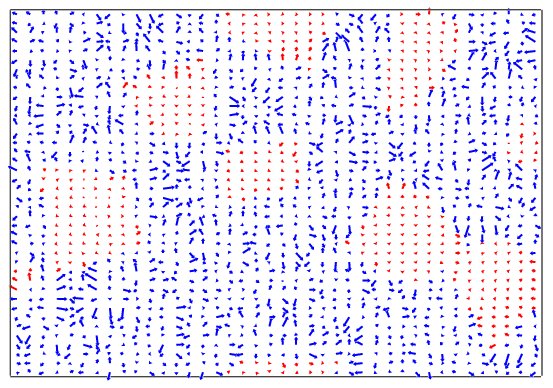
Snapshot of a simulation of PSN relaxor

A (110) plane through the PSN simulation box representing the projected local field (arbitrary units) at each Pb site in the plane. Chemically ordered regions (approximately circular) have small approximately homogeneous fields, and chemically disordered regions have larger more varied and disordered local fields. After [Tinte, Burton, Cockayne and Waghmare: Phys. Rev. Lett. 97, 137601 (2006)].

Frequency dependence of dielectric constant

$$\epsilon \left(\omega \right)-{\epsilon }_{\mathrm{\infty }}=\frac{1}{3{\epsilon }_{0}V{k}_{B}T}\left[⟨{\mathit{p}}^2⟩+i\omega {\int }_0^{\mathrm{\infty }}dt{e}^{i\omega t}⟨\mathit{p}\left(t\right)\cdot \mathit{p}\left(0\right)⟩\right]$$ where $\mathit{p}\left(t\right)$ is the total electric dipole moment in the supercell at time $t$,

$$\mathit{p}\left(t\right)=Z^{*}\sum _{\mathit{R}}\mathit{u}(\mathit{R};t).$$

Estimation of computational time

32x32x32 unit cells, $\mathrm{\Delta }t=2$ fs, [AMD64 1.8GHz dual core] or [SR11000 1 node = 16 cores]

1THz, $T=1$ps, 500 steps, 54 sec or 8.4 sec.

1GHz, $T=1$ns, 500,000 steps, 900 min. or 140 min.

1MHz, $T=1\mu$s, 500,000,000 steps, 620 days or 97 days

So, I am planning to calculate and compare $\epsilon \left(\omega \right)$ for $\omega /\left(2\pi \right)$ = 10M ... 10GHz.

Summary

• We developed "feram", a fast simulator for perovskite-type ferroelectric bulks and thin films
• Molecular dynamics (MD) simulation with first-principles-based effective Hamiltonian
• Phase transition of bulk ferroelectrics
• Thin-film capacitor: perfect and imperfect short-circuited electrodes
  • Striped domain structure is predicted
  • Hysteresis loops for epitaxially constrained and "free" BaTiO₃ film capacitors
• Investigations of relaxors with MD are proposed.

Thank you for your attention.